Most industrial operations are sitting on a goldmine and do not know it. Thousands of sensors are generating telemetry every second — vibration readings from motors, temperature curves from heat exchangers, pressure cycles from compressors — and nearly all of it is either discarded at the edge or stored in a historian that nobody interrogates until something breaks.
Gartner estimates that up to 70% of IoT-generated data is never analysed or acted on. Siemens and LNS Research put the average cost of unplanned manufacturing downtime at $260,000 per hour. These two numbers, read together, describe an enormous and largely avoidable problem.
This article explains how mature IIoT engineering teams bridge that gap: how they connect device-to-cloud infrastructure, what AI techniques actually detect fault signatures before failure, and how alerting can be built to give operators actionable signal rather than noise.
Why Most IoT Architectures Fail to Deliver Intelligence
The most common failure mode in industrial IoT is not a technology problem — it is an architecture problem. Teams bolt together point solutions: a SCADA historian here, a cloud bucket there, a dashboard someone built in a weekend, alerts that trigger on static thresholds. The result is a fragile stack that generates enormous amounts of data but delivers almost no insight.
Three structural gaps account for most of the failure:
1. Ingestion without schema contracts. Data flows in from dozens of device types and vintages, each with its own naming conventions, timestamp formats, and units. Without a normalisation layer and schema registry, the data lake becomes an unusable swamp within months.
2. Alerting built on static thresholds. A temperature alert that fires at 95°C is easy to configure. It is also nearly useless. Normal operating temperature for a motor under full load might be 92°C; for the same motor running at 20% load it might be 60°C. Static thresholds produce false positives under load and miss real problems in partial-load conditions. The result is alert fatigue: engineers learn to ignore the notifications, and the one genuine warning gets lost in the noise.
3. No model of normal. Predictive maintenance requires understanding what normal looks like for each device, across operating conditions, load states, and seasons. Without that baseline, you cannot detect deviation. Most teams never build it because they are busy managing the data infrastructure.
Fixing these gaps is the core of modern IIoT engineering.
The Five-Layer Stack That Actually Works
A production-grade IIoT data architecture has five layers, each with a specific job:
Layer 1: Device Connectivity and Protocol Handling
Industrial environments contain equipment from multiple generations and vendors. A modern compressor plant might have PLCs from Siemens and Allen-Bradley, SCADA historians from OSIsoft and Wonderware, newer IIoT gateways running MQTT, and legacy sensors that speak Modbus over RS-485.
The ingestion layer must handle all of them without requiring changes to the control layer. In practice this means:
- OPC-UA gateways for PLC and SCADA integration, using read-only data access to leave control operations untouched
- MQTT brokers (Eclipse Mosquitto, AWS IoT Core, Azure IoT Hub) for direct-connect IIoT devices and gateways
- Modbus polling agents for legacy sensors with no direct IP connectivity
- Protocol adapters for vendor-proprietary formats, translating into a canonical internal schema before data enters the pipeline
The canonical schema is critical. Every reading that enters the system should carry a device identifier, a sensor identifier, a UTC timestamp with millisecond resolution, a value, a unit, and a quality flag. Without this normalisation, every downstream consumer has to understand every upstream format, which is not maintainable.
Layer 2: Edge Computing and Local Inference
Not all telemetry decisions should be made in the cloud. For time-sensitive actions — emergency shutoffs, local alarming, bandwidth-constrained sites — edge compute is essential.
Edge runtimes such as AWS Greengrass, Azure IoT Edge, and lightweight Kubernetes distributions (K3s) run on industrial PCs or edge gateways in the plant. They perform:
- Local filtering and aggregation: Sending every raw reading to the cloud is expensive and often unnecessary. Edge agents compute rolling statistics (mean, standard deviation, min/max over a sliding window) and send summaries, escalating raw data only when anomaly conditions are flagged.
- Local inference: ONNX Runtime and TensorFlow Lite allow trained anomaly models to run at the edge with sub-millisecond latency. A compressor vibration anomaly detected locally can trigger a local alarm in milliseconds; waiting for a cloud round-trip might take seconds.
- Store-and-forward: When connectivity drops, edge agents buffer readings locally and replay them when the uplink recovers, ensuring no data gaps in the historian.
This architecture also reduces the blast radius of cloud outages. Sites can continue to monitor and alert locally even when the cloud data pipeline is unavailable.
Layer 3: Cloud Streaming and Batch Pipelines
Once data reaches the cloud, it enters the streaming layer. Apache Kafka (or managed equivalents like AWS Kinesis and Azure Event Hubs) provides the durable, ordered, replay-capable message bus that decouples producers from consumers.
The streaming layer serves several consumers simultaneously:
- Real-time anomaly detection models that score each reading as it arrives
- Time-series databases (InfluxDB, TimescaleDB, or cloud-native equivalents) that store raw and aggregated readings for dashboards and historical analysis
- Batch pipeline triggers that initiate model retraining when sufficient new data has accumulated
- Alert routing systems that translate model scores into actionable notifications
Apache Flink or Spark Structured Streaming handle stateful stream processing: joining readings from multiple sensors, computing rolling features, and applying windowed aggregations that models need as input.
Layer 4: AI Fault Detection and Predictive Maintenance Models
This is where raw telemetry becomes operational intelligence. The modelling strategy depends on what labelled failure data exists:
When failure history is sparse or absent — unsupervised anomaly detection:
- Isolation Forests are fast, interpretable, and work well for multivariate sensor data. They learn the distribution of normal readings and flag points that require anomalously few splits to isolate — statistically rare readings in the feature space.
- Autoencoders learn a compressed representation of normal operating states. Readings that the autoencoder reconstructs poorly (high reconstruction error) are anomalies. They handle high-dimensional sensor data well and can be trained unsupervised.
- Statistical baselines (rolling z-score, CUSUM) catch simpler drift patterns and are highly interpretable, making them useful as a first layer of detection even when ML models are in place.
When labelled failure history exists — supervised predictive maintenance:
- LSTM networks excel at learning temporal patterns in sensor sequences. They can identify the characteristic vibration signature that precedes a bearing failure, or the temperature ramp profile that precedes a thermal event, hours or days before the failure becomes visible on a single-sensor threshold.
- Gradient-boosted trees (XGBoost, LightGBM) trained on engineered features (rolling mean, rolling variance, spectral features from FFT) often outperform deep models on tabular sensor data and are significantly more interpretable.
- Survival models estimate remaining useful life (RUL) — not just whether a fault is likely, but how many operating hours remain before intervention is needed. This allows maintenance scheduling to be optimised rather than just reactive.
A mature predictive maintenance system layers these: unsupervised models run continuously on all devices, supervised models are deployed as failure history accumulates for specific equipment classes, and survival models drive the maintenance schedule optimisation.
Layer 5: Observability, Alerting, and Capacity Forecasting
The best models are useless if alerts are not actionable. Alert design is where most teams underinvest.
A tiered alerting architecture distinguishes:
- P1 — Immediate action required: Anomaly score exceeds a high threshold on a critical asset. Routes to on-call via PagerDuty or OpsGenie with a 60-second acknowledgement SLA.
- P2 — Investigation required within 24 hours: Anomaly trend is worsening but not yet critical. Creates a ticket in the maintenance system.
- P3 — Informational / trend watch: Model is flagging early-stage drift. Logged and summarised in a weekly digest for planned maintenance windows.
Suppress rules are as important as trigger rules. A model that flags the same anomaly 200 times during a known maintenance window trains engineers to ignore its output. Alert deduplication, maintenance window suppression, and alert correlation (grouping related alerts from the same asset into a single incident) are all part of responsible alerting design.
Capacity forecasting uses a different set of models. Rather than asking "is this device about to fail?", it asks "when will this system hit a limit?". Trend regression over historical utilisation (connection counts, throughput rates, storage fill rates, equipment load factors) projects forward against configurable breach horizons — typically 30, 60, and 90 days. Teams receive a weekly forecast: not an outage after the fact, but a projection with time to act.
A Real-World Example: Compressor Fleet Monitoring
Consider a compressed-air system serving a manufacturing plant — a common IIoT use case. The fleet of 12 rotary screw compressors runs 24/7 to maintain plant air pressure. Unplanned downtime costs the plant roughly £80,000 per day in lost production.
Previously, maintenance was calendar-based: compressors were serviced every 2,000 operating hours regardless of actual condition. This produced both premature servicing (replacing healthy components) and late servicing (missing developing faults between service intervals).
After an IIoT deployment:
- OPC-UA gateways connect to each compressor's existing PLC, reading discharge temperature, bearing temperatures, vibration (overall and band-pass filtered), inlet and outlet pressure, current draw, and oil temperature at 1Hz.
- Edge agents run on industrial PCs in the compressor room, computing rolling statistics locally and running a lightweight isolation forest that detects gross anomalies within seconds.
- Kafka streams readings to the cloud time-series database and to the real-time scoring service.
- LSTM models trained on the compressor OEM's failure case library and the plant's own historical service records score each compressor against 11 known fault signatures: bearing wear, oil contamination, valve fouling, filter clogging, and others.
- Survival models estimate RUL for each compressor, updated daily as new data arrives.
- Tiered alerts notify the maintenance team: P1 for imminent failure risk, P2 for "plan for service within a week", P3 for weekly trend summaries.
After 12 months, the plant reports:
- Two instances of incipient bearing failure detected 72+ hours before projected failure, allowing planned replacement during a shift changeover with zero production impact.
- Average service interval extended from 2,000 to 2,600 hours based on actual condition, reducing servicing cost by approximately 23%.
- Alert volume reduced by 60% compared with the old threshold-based system, restoring trust in the alert channel.
This is what the shift from reactive to predictive looks like in practice.
What Makes IIoT Projects Succeed (and Fail)
After multiple industrial IoT engagements, several patterns distinguish successful projects from expensive failures:
Brownfield integration is always harder than greenfield. Legacy SCADA historians, proprietary protocols, and network-isolated plant floors add weeks or months of integration work. Budget for it explicitly.
Data quality determines model quality. Models trained on sensor data where timestamps drift, calibration lapses, and sensor faults create systematic noise will learn the noise. A data quality pipeline — detecting stuck sensors, impossible values, calibration drift — is not optional.
Operational trust is earned slowly. Plant operators are rightly sceptical of new alert systems. Starting with P3 informational alerts, demonstrating accuracy over 2–3 months, then escalating to P1 alerting builds trust in a way that launching with full alerting on day one never does.
Edge compute pays for itself quickly. Cloud streaming costs for raw high-frequency sensor data can be significant. Edge aggregation that reduces egress by 80–90% pays back hardware costs within quarters.
The team mix matters. A successful IIoT project requires domain knowledge of the equipment being monitored alongside software engineering capability. Data scientists who have never worked with PLC data miss important signal characteristics; software engineers who have never worked in regulated plant environments make costly mistakes. The right team has both.
Getting Started: The First 90 Days
For teams beginning an industrial IoT programme, a phased approach reduces risk:
Days 1–30 — Connect and observe. Establish read-only connectivity to existing PLCs and historians via OPC-UA gateways. Get data flowing into a time-series database. Build dashboards. Do not build models yet; build understanding of the data.
Days 31–60 — Baseline and detect. Deploy statistical baselines and isolation forests across priority equipment. Configure P3 informational alerting. Let operators review the output and identify false positives before expanding scope.
Days 61–90 — Refine and escalate. Incorporate operator feedback to tune models and suppress rules. Graduate working detections to P2 status. Begin collecting labelled failure data for supervised model development in quarter two.
The 90-day programme delivers a functioning monitoring and alerting layer, operator trust in the system's output, and a data foundation for predictive models. It is not the finished product; it is the prerequisite for everything that follows.
The Bigger Picture: IIoT as Competitive Infrastructure
For manufacturers, utilities, and logistics operators, IIoT is increasingly a competitive differentiator rather than a nice-to-have. Operations that can predict and prevent failures, optimise maintenance spend, and forecast capacity constraints are structurally more efficient than those that cannot.
The technology to do this is mature and available. Apache Kafka, TensorFlow, LSTM networks, and cloud IoT managed services are production-proven at scale. The gap is not technology — it is engineering execution: the right team, the right architecture, and the discipline to start with data quality rather than model sophistication.
For organisations ready to move from data collection to operational intelligence, the path is clear. It starts with a single data source, a schema contract, and a team that understands both the plant floor and the cloud.
Related Reading
- IoT Sensor Data Processing and AI Fault Detection Services — How CodeCones builds end-to-end IIoT engineering from sensor ingestion to AI fault detection.
- Data Engineering Services — The data pipeline and streaming infrastructure that underpins industrial intelligence.
- Custom AI Development — Bespoke machine learning models for fault detection, predictive maintenance, and anomaly detection.
- Get in Touch — Talk to a CodeCones IoT engineer about your connected operations.
- SRE consulting for telemetry and incident response — Connect operational signals to reliability targets, alert ownership and recovery planning.
About CodeCones Team
The CodeCones team consists of enterprise software architects, platform engineers, and AI solution specialists building outcomes-driven technology for global businesses.
View full profile →Key Takeaways
- Up to 70% of IoT-generated data is never analysed; the gap between data collection and operational intelligence is an architecture problem, not a technology problem.
- A five-layer IIoT stack — device connectivity, edge compute, cloud streaming, AI modelling, and alerting — is the blueprint that separates monitoring systems from intelligence systems.
- Static threshold alerting produces alert fatigue; AI models that learn normal device behaviour per operating condition are required for actionable, low-noise fault detection.
- Unsupervised anomaly detection (isolation forests, autoencoders) works without labelled failure history; supervised LSTM and gradient-boosted models are added as failure data accumulates.
- Tiered alerting with maintenance window suppression and deduplication is as important as the underlying models; operators who trust the alert channel act on it.
- Edge computing reduces cloud streaming costs by 80-90% on high-frequency sensor data and allows local inference to operate independently of cloud connectivity.
- The first 90 days of an IIoT programme should focus on connectivity, data quality, and baseline statistical detection — not model sophistication.
References
- [1]Gartner — IoT Data Usage Statistics
- [2]Oxford Economics — The Hidden Costs of Downtime
- [3]McKinsey Global Institute — The Internet of Things: Mapping the Value Beyond the Hype
- [4]IEEE — A Survey on Industrial Internet of Things: A Cyber-Physical Systems Perspective
- [5]AWS — AWS IoT Greengrass Developer Guide
- [6]Apache Kafka — Kafka Use Cases in IoT and Telemetry
- [7]Towards Data Science — Anomaly Detection for Time Series with Machine Learning
- [8]Fortune Business Insights — IoT Market Size, Share & Industry Analysis